iFit User Interface

To avoid the need to write a script for every use a Graphical User Interface (GUI) was developed for iFit. This also helps to facilitate spectra acquisition and real-time analysis. This section will outline the setup and use of the GUI for both real-time and post analysis. This will apply for running the GUI with Python or from an executable file.

GUI Overview

When the GUI is launched the user is presented with the screen shown in Fig. 1.

This has three main sections:

1. Program Controls

2. Program Outputs

3. Graphs and Settings

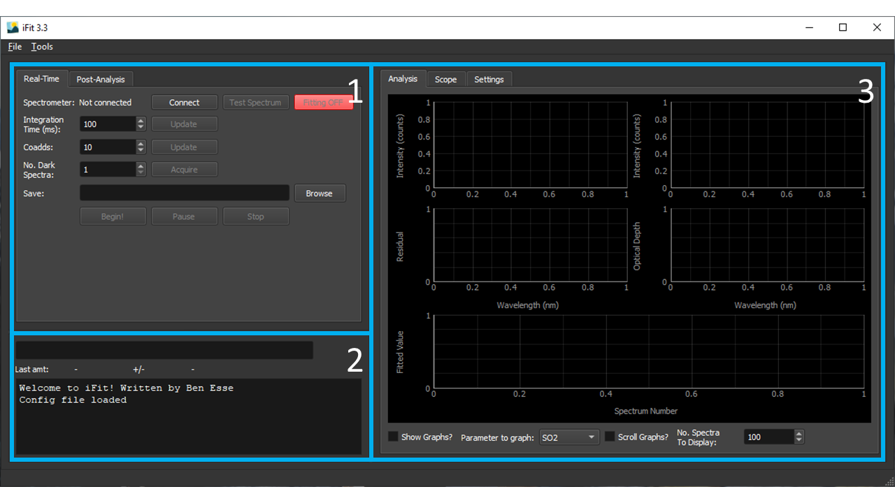
Figure 1: The main GUI interface

Program Controls

The program controls are slit into two tabs, Real-Time and Post-Analysis (Fig. 2). As suggested by the names, the Real-Time tab handles spectra acquisition and real-time analysis, while the Post-Analysis allows the processing of already acquired data.

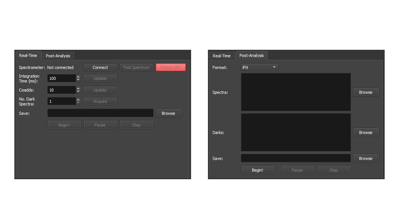
Figure 2: GUI controls

Real-Time Controls

Item	Description
Spectrometer	Displays the serial number of the connected spectrometer. Connect/Disconnect to the spectrometer by clicking Connect
Test Spectrum	Reads a single spectrum to test the connection and acquisition settings. This spectrum is not saved but displayed on the Scope plot
Fitting ON/OFF	Toggles real time analysis of spectra as they are recorded
Integration Time (ms)	The integration time of each individual spectrum in ms. Use the Update button to push to the spectrometer
Coadds	Number of individual spectra to average to form a measurement. Note that averaging is done in software not onboard the spectrometer. Use the Update button to push to the spectrometer
No. Dark Spectra	The number of dark spectra to record. Begin acquisition of dark spectra by clicking the Acquire button. Dark spectra are saved to a subdirectory in the save folder called Dark. Note that each read creates a new folder (numbered sequentially)
Output Folder	Path to the folder to contain the measurement results. This includes measurement spectra (stored under /save/path/spectra/), dark spectra (stored under /save/path/spectra/dark) and analysis outputs
Begin!	Launches continuous spectra acquisition (and simultaneous analysis if Fitting ON)
Pause	Paused the acquisition/analysis
Stop	Ends the acquisition/analysis

Post-Analysis

Item	Description
Format	Format of the spectra files to read
Spectra	Measurement spectra files. Can be selected using a File Dialogue with Browse
Darks	Dark spectra files. Can be selected using a File Dialogue with Browse
Output File	Location to save the output .csv file to
Begin!	Launches spectra analysis
Pause	Paused the analysis
Stop	Ends the analysis

Program Outputs

This frame contains a progress bar and text box to display program progress and any info or error messages.

Graphical Display

This frame contains the graphical output of the program. The Analysis tab shows the results of spectral fits, while the Scope tab shows the acquired spectra.

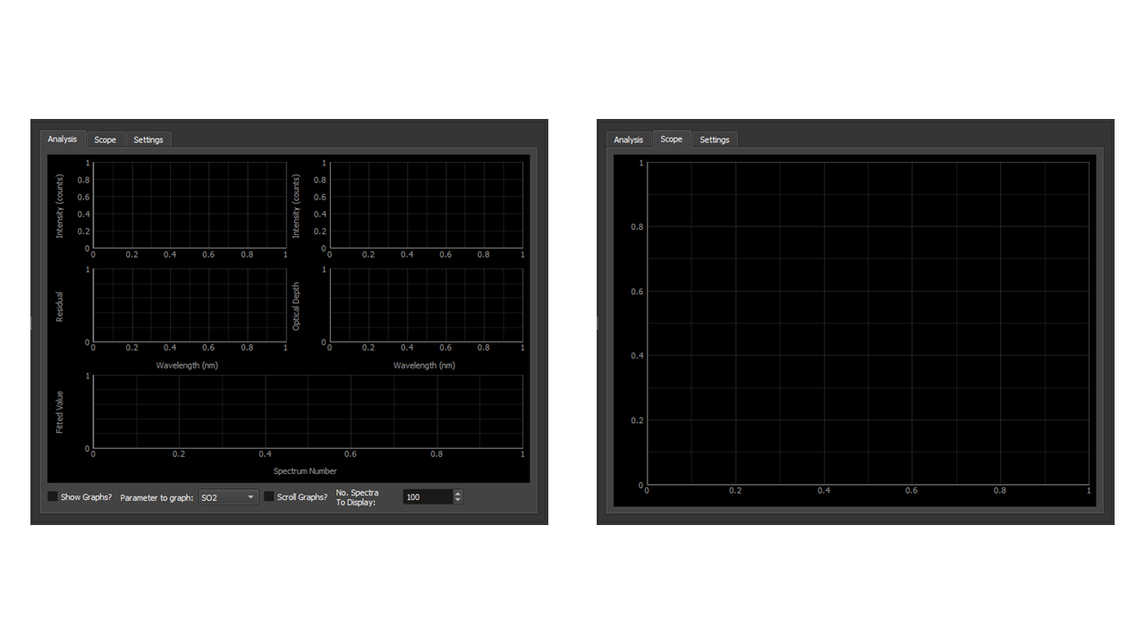
Figure 3: GUI graphical outputs

The bottom of the Analysis tab has a number of options for the graphs.

Item	Description
Show Graphs?	Toggles whether graphs are plotted or not. Plotting graphs requires some computational resources so analysis can slow as a result. This impact is lessened if the limits of the graphs are fixed (this can be done by hand)
Parameter to graph	Sets the parameter to display in the optical depth and parameter plots. These display the synthetic and measured optical depths, and the fitted parameter value respectively.
Scroll Graphs?	Toggles whether the bottom graph scrolls or not. If not then all data points are show, which can significantly slow down the program if the number is large. Other wise the number of spectra to display is given in the No. Spectra To Display option

Program Settings

The final tab contains the program settings. These include the fit window and quality controls, any spectral pre-processing steps required and the parameters to include in the fit.

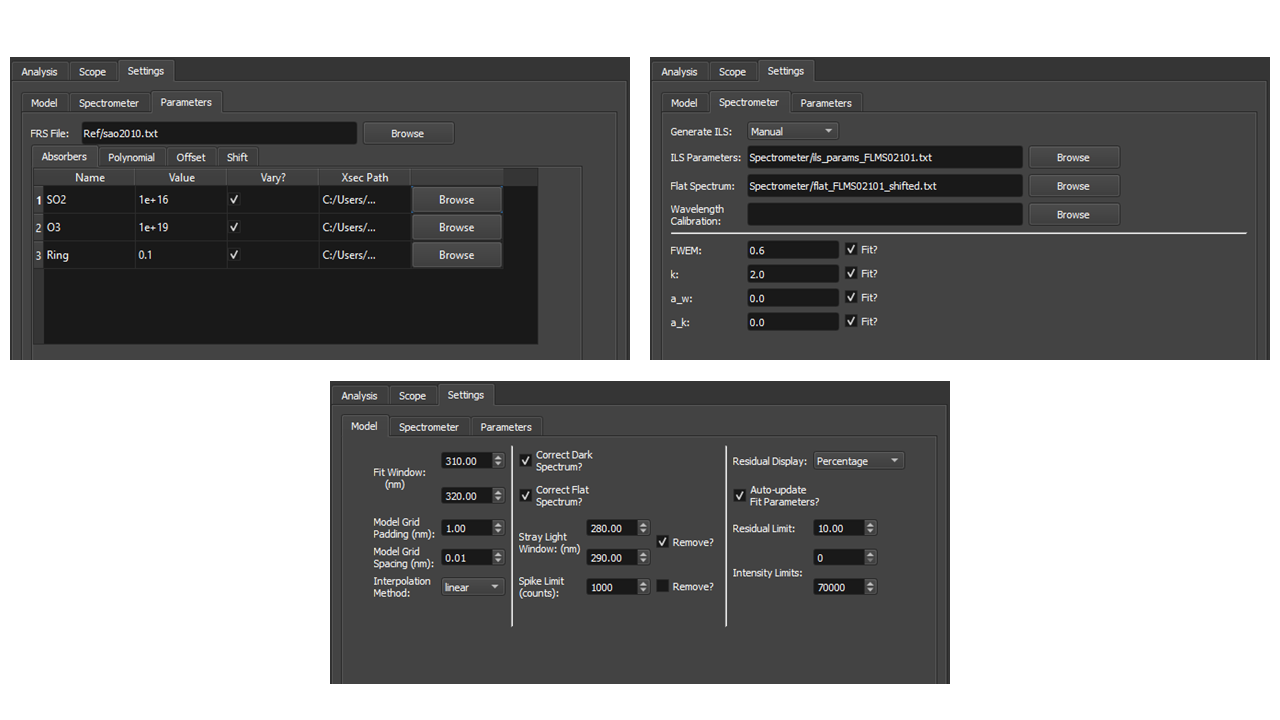
Figure 4: GUI settings

The settings are split into three tabs:

Model

Item	Description
Fit Window	The wavelength window in which o perform the fit
Model Grid Padding	The amount to pad the model grid in order to avoid edge effects from the ILS convolution
Model Grid Spacing	The spacing on which the model grid is formed
Interpolation method	The method to use in each iteration of the model fit to interpolate the model spectrum onto the spectrometer wavelength grid. cubic is more accurate but linear is faster and more stable
Correct Dark Spectrum?	Controls whether the dark spectrum is subtracted from the measured spectrum during the spectrum pre-processing step
Correct Flat Spectrum?	Controls whether the flat-field spectrum is removed from the measured spectrum during the spectrum pre-processing step
Stray Light Window	The wavelength window over which to average the stray-light intensity. This is subtracted from the measured spectrum in the pre-processing step if the Remove checkbox is selected
Spike Limit	Sets the limit at which to remove hot or dead pixels. Defined as the intensity change between neighbouring pixels
Residual Display	Controls how to display the residual, either as a percentage of the measured signal or in absolute intensity units
Auto-Update Fit Parameters	Controls whether the first guess fit parameters used are updated with the previous fit’s optimised parameters. This speeds up analysis, but can lead to the fit getting stuck in a local minimum, especially for poor quality data
Residual Limit	Sets the maximum value the residual can be to be classed as a good fit. Bad fits also reset the first guess parameters if Auto-Update Fit Parameters is on. Note this value should be changed if switching between Percentage and Absolute residual display
Intensity Limit	Sets the limits on intensity in the fit window for which the fit can be considered good. Bad fits also reset the first guess parameters if Auto-Update Fit Parameters is on.

Spectrometer

Item	Description
Generate ILS	Controls how the instrument line shape is handled. Params uses fixed parameters read from a text file defined at ILS Parameters. These should be the FWEM, k, aw and ak values respectively, each on a new line. File uses a directly measured lineshape read from ILS Parameters. Manual uses the parameters given in this tab, with the option to fit them if desired.
ILS Parameters	File the contains either the ILS super-Gaussian parameters or the directly measured lineshape to use
Flat Spectrum	Path to the flat spectrum to use. Should be a file with two columns delimited with a tab. The first is intensity and the second is the flat-field response.
Wavelength Calibration	The wavelength calibration to use if none are given in the spectra files.
FWEM, k, aw, ak	The super-Gaussian parameters to use if Generate ILS is set to Manual. These parameters can also be fitted if desired.

Parameters

This tab sets up the fit Parameters through a series of tables. For each table rows can be added or removed by right-clicking on the table.

The Absorbers table controls the absorbing species included in the fit, such as gases and Ring. Each absorber Parameter has a name (which must be unique), a value, a control on whether it is fitted or fixed and a file from which to read the cross-section. The cross-section file should have two columns, one for the wavelength and one for the cross-section efficiency.

The Polynomial, Offset and Shift tables control the polynomial parameters for the fitted background polynomial, intensity offset and wavelength shift/stretch included in the fit.